DEM
A DEM (Digital Elevation Model) contains points with elevation data. DEM Data are based on LIDAR (Light Detection and Ranging) technology measurement, also known as Airborne Laser Scanning. There are DEM with point data arranged in a regular grid with a constant distance between the points. This distance is called cell size. Other DEM contain data points arranged irregularly (cloud-model).
- Read more about this topic: http://en.wikipedia.org/wiki/Digital_elevation_model

A laser beam splits as it hits objects. The result are multiple returns. The difference between first and last return can show object height. The last return doesn’t always reach the ground.
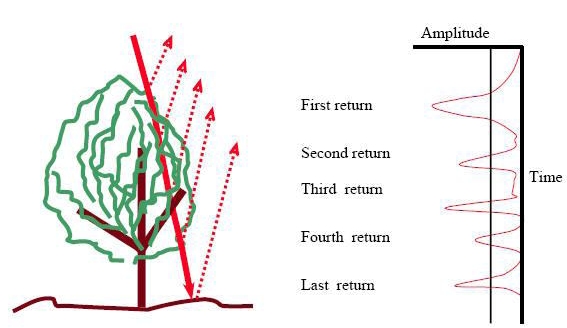
- Source: Lohani, Bharat. Airborne Altimetric LiDAR: Principle, Data Collection, Processing and Applications.

DEM Import Wizard
Read more about importing DEM file on the page DEM Import Wizard.
Open 


Open an OCAD DEM file (*ocdDem). OCAD 12 can also open ocdDems created in OCAD 11.
Show Frame
Shows blue rectangle with the extent of the loaded DEM.
Resize
Resize the loaded OCAD DEM file (make a subset) and save it as a new OCAD DEM file.
Info
Shows information about OCAD DEM file.
![]() When moving the mouse cursor over the file name then the file name with path appears.
When moving the mouse cursor over the file name then the file name with path appears.
Close
Close OCAD DEM file.
Merge DEM

Choose Merge from DEM menu to merge two different DEMs.
- DEM 1: Choose the first DEM.
- DEM 2: Choose the second DEM.
![]() The two DEMs must have the same cell size.
The two DEMs must have the same cell size.
Calculate DEM Difference

- Choose Calculate DEM Difference from DEM menu.
- The Calculate DEM Difference dialog box appears.
- Add Upper DEM = DSM data file
- Add Lower DEM = DEM data file
- Click OK.
To visualize the DEM difference choose Classify Vegetation Height
![]() The extent of the Upper DEM and Lower DEM can be different. OCAD takes the overlapping area for the new DEM.
The extent of the Upper DEM and Lower DEM can be different. OCAD takes the overlapping area for the new DEM.
![]() The cell size of Upper DEM and Lower DEM can be different. OCAD takes the cell size of Upper DEM for the new DEM.
The cell size of Upper DEM and Lower DEM can be different. OCAD takes the cell size of Upper DEM for the new DEM.
Example
This is an example to show what can result from the Calculate DEM Difference function.
This is a DTM (Digital Terrain Model) with a cell size of 5m shown as hypsometric map:

The next picture shows the DSM (Digital Surface Model) of the same area with a cell size of 2m as hypsometric map. The buildings (northern part) and forest (south western part) are slightly visible.

The next picture shows a Difference DEM with a cell size of 2m shown as raster background map after calculating the DEM Difference. In addition, heights were colored using the Classify Vegetation Height function.

- The area with no difference of the DTM and the DSM are displayed white.
- A height difference up to 15m appears red.
- The greater the difference, the greener an area appears.
When moving the mouse cursor over the map the difference is shown in the Status Bar.
Data source: Test data Wabern from swisstopo.
Create Contour Lines
- Choose Create Contour Lines from DEM menu.
- The Create Contour Lines dialog box appears.

This function calculates contour lines based on the loaded DEM.
This function can take a lot of time. OCAD starts to calculate the contour lines from the lowest elevation (minimun contour). During the calculation process the current elevation is shown in the left status bar.
- Define 1-3 contour intervals (for example 1m, 5m, 25m) and a pre-selected line symbol (according to the first three line symbols in the settings) for each type appears (can be changed).
 Contour interval values can be entered manually or chosen from the list.
- Specify the minimum (lowest) and maximum (highest) contour for the calculation.
- Activate the option Split DEM into tiles to speed up this calculate process. In this case OCAD splits the dem into small tiles and calculates tile by tile. Finally the contour lines are also splites at the tile borders. It is not visible on the screen but you see it when selecting a contour line. Use the Merge Contour Lines By Selected Symbols function to merge the contour lines if needed.

The selected contour line is cutted at the tile borders.

Create Hypsometric Map

- This function calculates a grayscale or colored hypsometric map as GeoTIFF file.
- Optionally it is directly loaded as background map.
Two different types of hypsometric maps can be edited:
- Grayscale hypsometric map
- Colored hypsometric map

Create Hill Shading

- This function calculates a shaded relief picture (hill shading).
- There are two calculation methods available:
- Slope shading is optimized to see outlines of features like paths in a slope.
- Slope shading combined with oblique light shading is the recommended method if the hill shading should be used as a background relief of a map.
Optionally the calculated hill shading is directly loaded as background map.
- Aside from the chosen method, there is to define the Resolution and the Interpolation mode (if chosen).
- The default interpolation mode is Bicubic, but there are 7 other algorithm.
- Additionaly an Azimuth and a Declination of the light source has to be set. Standard settings are 315° (north-west) and 45°.
An Exaggeration factor of 4 is pre-selected and can be altered.
The Preview... button allows you get a first impression of the current setting for your hillshading and can be use to optimize it.
- Click and move with the left mouse button allows to pan the current view.
The Preview... button is only enabeld when importing a dem grid file or an ocddem is already loaded. This function is disabled when importing las/laz files.
![]() To detect point and line objects like paths or watercourses from DEM we recommend using the same resolution as the DEM. To create a relief and if the DEM cell size isn’t high then we recommend to set a smaller resolution.
To detect point and line objects like paths or watercourses from DEM we recommend using the same resolution as the DEM. To create a relief and if the DEM cell size isn’t high then we recommend to set a smaller resolution.
![]() The default export file format is JPEG and creates an 8 bit JPEG with in grayscale and a world file with the geo reference. If you decide to export the file in TIFF-format, only with resolution option ‘DEM cell size’ then OCAD creates an 8 bit grayscale tiff with color palette. Otherwise a 24 bit RGB tiff.
The default export file format is JPEG and creates an 8 bit JPEG with in grayscale and a world file with the geo reference. If you decide to export the file in TIFF-format, only with resolution option ‘DEM cell size’ then OCAD creates an 8 bit grayscale tiff with color palette. Otherwise a 24 bit RGB tiff.

Error Message Bitmap is too big
The size of the hill shading image is limited. If this error message appears please enter a bigger value for the interpolation.
Calculate Slope Gradient

- Choose Calculate Slope Gradient from DEM menu.
- The Calculate Slope Gradient dialog box appears.
Select one of two different methods:
- Continous (<x° = grayscale / >x° = black)
- Black/White (<x° = white / >x° = black)
The resulting picture can be used to identify cliffs an rock faces. The result can sometimes be significantly improved with a slight adjustment of the gradient (between 42-45 degrees).
Slope gradient also shows paths or relief features independent from a azimut like the Hill Shading.

Classify Vegetation Height

Choose Classify Vegetation Height from DEM menu.
There are two different options to show vegetation height classification:
- Gray scale classification with options: Linear, Quadratic negative, Quadratic positive
- Colored classification: Define classes with a height and color range
- - Split a class into two classes by clicking the Split class button
- - Remove a class by clicking the Remove class button
- - Load the settings from a text file by clicking the Load button
- - Save the settings to a text file by clicking the Save button
- - Reset the classes and colors to the default settings by clicking the Reset classes to default button

Merge Contour Lines By Selected Symbols
- Select the contour line symbols
- Choose Merge Contour Lines By Selected Symbols from DEM menu.
- The Merge Contour Lines By Selected Symbols dialog box appears.

Create Profile

Find more information about this function on the DEM Profile page.
Export
- Choose Export from DEM menu.
- The DEM Export dialog box appears.

The function exports the loaded DEM file to the following formats:
- ESRI ASCII Grid
- ASCII Grid XYZ
- OCAD 11 DEM
Select Create tiles for large DEMs to create tiles fron 1001x1001 points.
The OCAD 12 DEM's cannot be opened in OCAD 11. This export function creates a OCAD 11 compatible DEM.
ocdLas File
Learn more about the ocdLas File functions on the ocdLas File page.
Back to Main Page
Previous Chapter: Printing Maps
Next Chapter: GPS